sciences de la vie et de la Terre
 s'identifier
 portail personnel ETNA
espace pédagogique > disciplines du second degré > svt > transversalité > DNL
GPS tracking of the european lithosphere deformations
mis à jour le 06/11/2003
Using GPS data to evaluate vertical and horizontal deformations of the lithosphere and performing analogical modellings of a few deformation phenomena.
mots clés : GPS, lithosphere, deformation, isostasic equilibration, collision, tectonic, Tice
Présented by Chloé ANFRAY, Ronan CALVEZ, Guillaume DEFOIX, Vincent LE GALL, Romain NEUVILLE, Clémence PAGNOUX and Victor PRAUD.
Teachers : François CORDELLIER, Biology and geology, Annick LANGLAIS, Mathematics, Bertrand MABILLAIS, Physics and chemistry.
With help of Mélanie GUILLET (English teacher) for translation.
 |
How can we represent and simulate the European lithosphere’s deformations after measuring them with computed GPS data ? |
Project origin :
| Our geology courses include GPS data treatments. Our aim was to complete our knowledge of the European tectonic plates internal deformations and to be as precise as possible. During a geological excursion we used GPS receivers to localise outcrops. Besides we know that accurate GPS data are used by geologists to measure plates’velocities. We thought it would be possible to use the same data to evaluate vertical and horizontal deformations of the lithosphere. After that, we tried to perform analogical modellings of a few deformation phenomena. For example, Archimedes’ principle can be used to explain the post-glacial rebound of the northern part of Europe. |
Summary :
Data and proceedings
Latitudinal and longitudinal absolute velocities
European plate horizontal internal deformations
Lithospheric vertical movements
Modelling post-glacial rising
Modelling alpine orogenesis
The GPS
The GPS system (Global Positioning System) is used
to determinate the position of a point with a high precision. Receivers
from the station or mobile compute the position using a satellite constellation
running around the whole Earth. The satellites broadcast a radio signal
to the receivers. |
With agrement of EUREF : http://epncb.oma.be |
Velocities are calculated following tree directions
: latitude (Vel lat), longitude (Vel long) and altitude (Vel alt).
|
 |

Data proceeding
|
|
We downloaded data from the NASA web site : http://sideshow.jpl.nasa.gov/mbh/series.html They are in text format. We had to copy them in a spreadsheet in order to sort and select them. Relative speeds can also be computed on this spreadsheet. |
 |
We selected the European receiver’s lines and
drew the velocities as vectors by adding the latitudinal velocity vector
to the longitudinal velocity vector for each measurement point. |

Different maps were drawn in the same way : Horizontal velocity, horizontal relative velocity and vertical velocity.
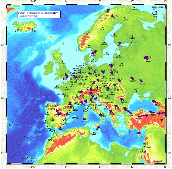
The european lithospher horizontal movements
 |
This map shows the velocity of each receiver in Europe. We notice that the European plate moves roughly toward the North -East 6 or 7 centimetres per year. However the receiver in Ankara moves toward the North because it is fixed to the Anatolian plate and not to the European one. Comparing the velocities of the different parts of the European plate raises a question. Receivers are fixed to a rigid lithospheric
plate. Why don’t they move exactly with the same velocities
and directions ? With autorisation of the EUREF website : |
To answer this question we have to calculate the velocity of each point compared with a fixed one.
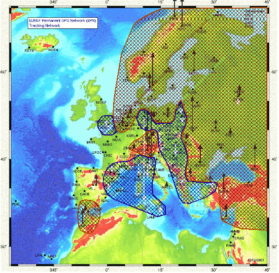
The european plate internal deformations
Using the excel spreadsheet, we can calculate the relative velocities of each point compared to another one of the European plate which is now considered as fixed. Latitudinal and longitudinal relative velocities are given by subtractions following this rule :
Relative lat. vel. = studied point absolute lat. vel. -
fixed point absolute lat. vel.
Relative long. vel = studied point absolute long. vel. - fixed point absolute
long. Vel.
Relative velocities vectors are drawn by composition of latitudinal and longitudinal relative velocities vectors.
 |
For this first map the fixed point was chosen in
Trömsø in northern Norway. |
 |
For this map the fixed point was San Fernando in southern Spain. The same phenomenon can be found in South eastern Europe and the Alps |
 |
The fixed point for this map is the NPDL receiver
in the town of Teddington (UK)
|
Lithospheric rocks are rigid. We must look for movements of vertical deformations to understand the lithospheric plate shortening mechanism.
The european plate vertical movements
 |
We worked only on the vertical velocities
(vel Alt) of the GPS stations |
On the European map, white arrows correspond to subsiding movements and black arrows to rising movements.
 |
Subsiding and rising movements are both present in Europe with very different values.
|
 |
To emphasize global trends, rising zones (in red)
and subsiding zones (in blue) are drawn on the map. |
Some bibliographical researches provide us with hypothese about the rising and subsiding mechanisms. For Scandinavia, post-glacial rebound could be pleaded and orogenic movements could explain the Alps rising. A lot of hypothese could explain subsiding movements such as rifting, sediment accumulation, water pumping, etc.
The measured rising movements in Scandinavia can be more
than 6 mm/y. It can result of artic Iceland melting at the end of the Würm
glacial time. Excess of weight due to ice disappeared at that time and the lithosphere
began to rise following Archimedes’ principle. This phenomenon is called
“isostatic rising”. The very high asthenospheric mantle viscosity
makes it very slow and this isostatic rising is still going on nowadays.
Analogical modellisation is possible if we use a high viscosity fluid to simulate
the ductile asthenospheric mantle. We operate with a wood block floating on
wallpaper paste. First the woodblock is sunk in the paste with the hand. It
looks like the effect of iceland weight on the lithosphere. Then the block is
slackened simulating ice melting. The block rises very slowly and this rising
lasts for a long time after slackening.
Rising was followed by digital recording and a picture was
extracted every 15 seconds.
 |
At t = 0 the wood block is slackened. The GPS is symbolised by a bullet on three legs. Relative altitude(A) is 0 mm |
 |
t = 15 s A = 3 mm |
 |
t = 30 s A = 8 mm |
 |
t = 45 s A= 10 mm |
 |
t = 60 s A = 12 mm |
 |
t = 75 s A = 15 mm |
 |
t = 90 s A = 19 mm |
 |
t = 105 s A = 22 mm |
 |
t = 120 s A = 25 mm |
 |
t = 135 s A = 30 mm |
 |
t = 150 s A = 32 mm |
 |
t = 165 s A = 35 mm |
 |
t = 180 s A = 37 mm |
Altitude according to time can be measured on the scale of the block side.
Drawing the curve of altitude according to time shows that the function is affin. When approaching equilibrium the rising slows down and stops. As Scandinavia is still rising we concluded that equilibrium has not yet been reached.
 |
This isostatic phenomenon can also explain why central European plains and the Italian Piedmont subside under sediment’s weight. But we can’t use it to explain why the Alps rise strongly in their central part.
Modelling of the alps orogenesis
Nowadays the central Alps rise along the border of two old tectonic plates. The alpine ocean disappeared and the two continental crusts are now joined but collapsing movements from South East to North West are in progress. They could be responsible of the mountain rising
 |
Layers of colored plaster are set in a transparent box with a piston on one side to represent a part of crust with sedimentary rocks. |
 |
Pushing the piston from right to left deforms the layers. It simulates the movement of South eastern Europe toward North West. |
 |
Rising and shortening are observed. Inverse faults and folds appear. This experiment confirms our hypothesis as faults and folds are really observed in the Alps. |
 |
The shortening increases the crustal thickness and the GPS receivers fixed to the crust record a rising movement. |
In spite of this good result our simulation is not perfect because it cannot simulate at the same time the isostatic adjustment due to the thickening of the crust.
Elèves du lycée Jean Perrin
information(s) pédagogique(s)
niveau : 1ère S, Terminale S
type pédagogique : production d'élève
public visé : enseignant, élève
contexte d'usage : atelier, classe, espace documentaire, laboratoire, salle multimedia
référence aux programmes :
Structure, composition et dynamique de la Terre
sciences de la vie et de la Terre - Rectorat de l'Académie de Nantes